Japanese beetle project
Japanese beetles (JB) are an invasive species in the United States. At the moment, the most effective controls are conventional insecticides. Although efforts were made to introduce parasitoids from their native range (classical biocontrol), they were not successful at establishing populations large enough to control JB. Dave Smitley's lab at Michigan State University has been studying the effects of Ovavesicula popillae (originally discovered by Andreadis and Hanula, 1987) on JB populations. Their work has shown significant reductions (up to 75%) in JB populations over 18 years.
In this study, we aimed to detect Ovavesicula popillae in Minnesota and quantify the abundance of Japanese beetles. We also want to control for other factors that may explain abundance, such as weather conditions and greenery (measured using NDVI).
Abbreviated methods
Sampling design
Japanese beetles were sampled every two weeks at 44 sites in the Twin Cities metro area. A Japanese beetle pheromone trap was set up and beetles were collected 24 hours later. From the beetles collected, we measured the number volumetrically using a graduated cylinder. For ~30 samples, we collected both volumetric data and manually counted beetles to perform a linear regression and create an equation to convert volume to quantity. This equation was used in data manipulation (Figure 1).
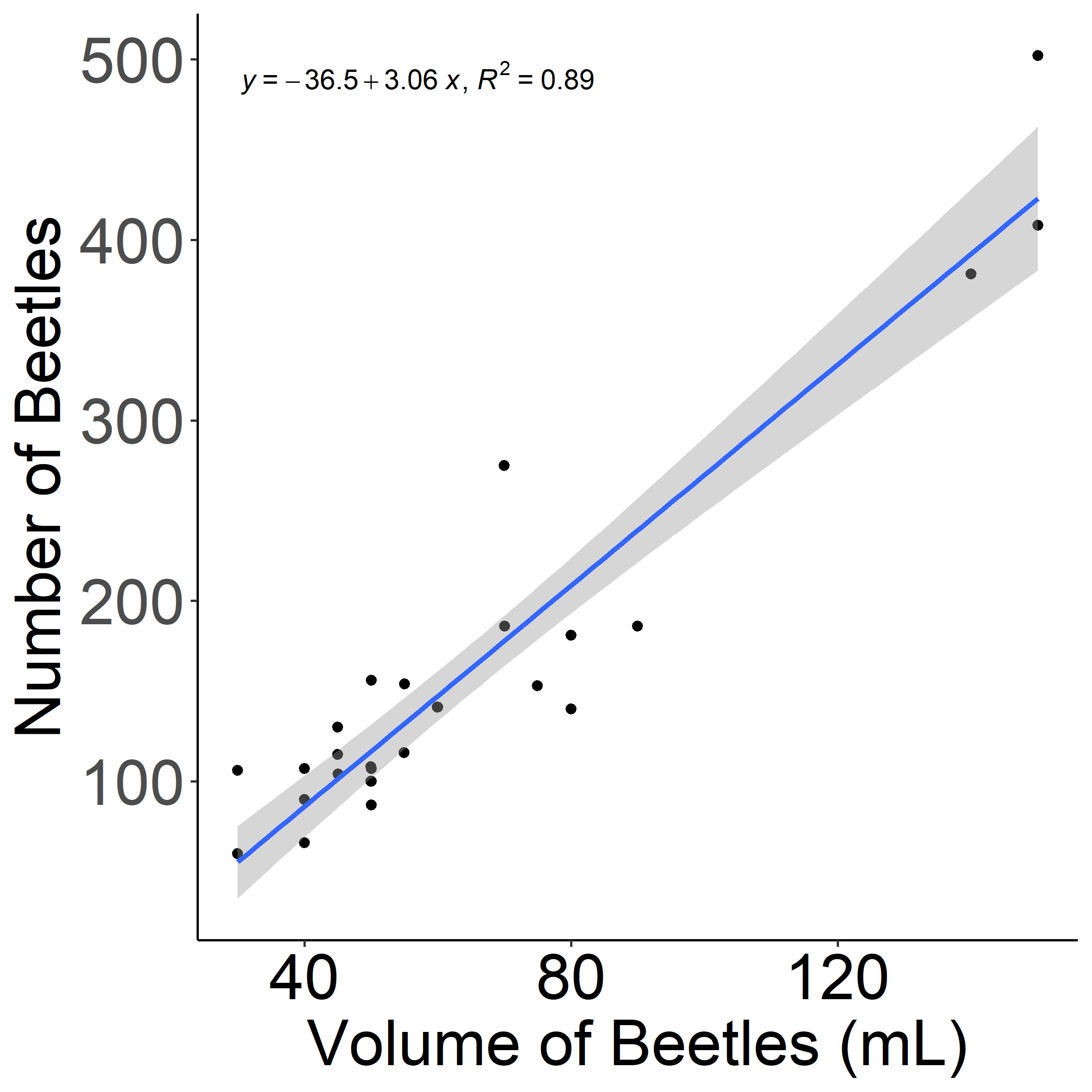
Figure 1: Linear regression for volume x quantity of Japanese beetles.
Quantification of Ovavesicula popillae
Once volumetric and/or count data were taken, Japanese beetles were separated into either saline or ethanol (following methods from Smitley et al. 2022). Japanese beetles stored in saline were then dissected and Ovavesicula popillae spores were counted using microscopy techniques (such as Cantwell, 1970). Beetles stored in ethanol had DNA extracted and spores were quantified using qPCR.
Remaining data used in the final analysis were collected using data mining techniques in Python.
Data manipulation in R
Large scale data is rarely clean, so to make this dataset usable, data manipulation is required. Our datasheet includes information for the number of beetles collected for saline, ethanol, and volume (or count) data. The data need to be subsetted to only show volume/counts. Then, samples that were too small for volumetric measurement need to be replaced by the count. To accomplish this, I wrote a for loop where NA values for beetle counts are replaced by volumetric data.
Using Python to collect environmental covariates
Weather data
To collect weather data, I chose to use Meteostat, an open source weather and climate data vendor, due to their thorough documentation and ease of use. I hypothesized that Japanese beetle counts will depend on the weather (temperature, humidity, rainfall, etc.) both while traps were deployed as well as the 24 hours before traps are deployed. For brevity, I will only focus on the 24 hours while traps were deployed here. Meteostat's weather data is easily collectible using their API. Unfortunately, our date and time are in the wrong format. To communicate with Meteostat, we need year, month, and day in separate columns along with hour and minute in distinct columns as well. To do this, I split dates and times (for both trap deployment and collection) into disctinct columns using str.split in Python.
The data have xy coordinates, but Meteostat requires a z coordinate (i.e. elevation). for convenience, I could pick a number close to most site's elevations, but doing this will still make some sites undefined. I used Open Topo Data instead, so that each site would have the correct elevation. I made a loop that gives each line's coordinates and receives the elevation. After, this elevation will be appended to an array, and then the array will be added as a column in the dataframe.
The last step is to feed Meteostat time data and receive weather data during the time our traps were deployed. The start time for weather data will be the exact time we deployed the trap and it will end when we picked up the trap and counted beetles.
We now have temperature, humidity, rainfall, wind speed, and wind direction to use in our analysis. This should help control for some of the variability in the data. Our code is also now easily editable to account for other hypotheses, such as the weather 24 hours prior to sampling having an effect, or the average weather for the year prior.
Below is the effect of our weather data on beetle abundance.
.png)
Figure 2: Effect of weather variables on the model residuals. Temperature and wind speed have a positive effect on the number of beetles, while humidity and rainfall have a negative effect.
Remote sensing data
To determine the effect of greenness on beetle abundance, I am going to collect satellite data from the Sentinel 2 mission. This is a good option because it has a 20 meter resolution, which will be useful for our small study sites. I am interested in whether the vegetation (quantified as average NDVI) predicts the abundance of beetles or infection prevalence of Ovavesicula. These data should be on a per plot basis, which requires conversion of xy coordinates to polygons. There are shapefiles for land use in the Twin Cities, and in R, I used the coordinates to remove all polygons except for those that were used in this project. This leaves us with shapes that outline each study site.
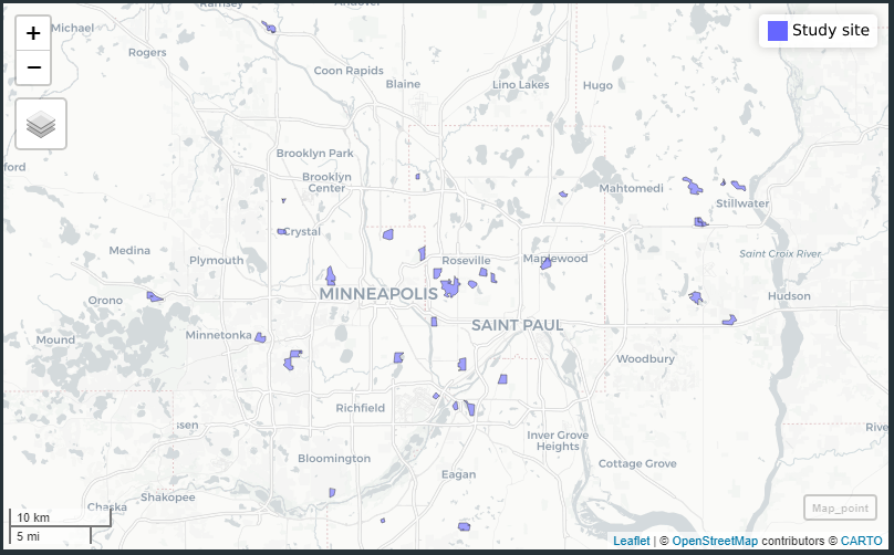
Figure 3: Study sites used in this project outlined in polygons. Data for land use was pulled from Minnesota Geospatial Information Office
To access the data I will use Google Earth Engine. Images can be collected from the time of year we are interested in quantifying NDVI from. We will need the total boundary of our area of interest to select the images from the satellite. First, we set up Earth Engine. The area of interest is determined and passed into Sentinel 2 image collection. Once this is done, we can pick dates and filter the metadata by cloud percentage. Then we make a list of our images to pull from shortly.
I made a quick map to make sure our images look correct. First, I calculated NDVI from bands 8 (NIR) and 4 (Red). I used the folium package in Python to make a map that can be moved around and ensure we are selecting the correct image. Since there is not one image that contains all of our sites, I will make calculations based on 3 images. Below is an example of one of the images.
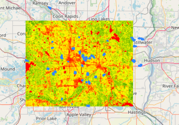
Figure 4: Imagery from Sentinel 2 satellite, mean NDVI calculated from bands 8 and 4 (NIR and red). Given that some sites fall outside of our bounds, use multiple images to composite NDVI calculations.
Next, we can make a for loop that exports those images to Google Drive.
Finally, we can make one last loop that opens those images, applies a crs, and calculates the min, max, mean, std, and count of NDVI. All those stats get exported into a dataframe, and we can then open in R to do our statistical analysis.
This dataframe now has statistics for NDVI at every site, we can merge with our other dataframes in R. Below is the mean NDVI for our sites. We can also use the standard deviation and count to calculate standard error, which is a more useful statistical for variability. We also now have the code to select multiple points in time that we can compare to.
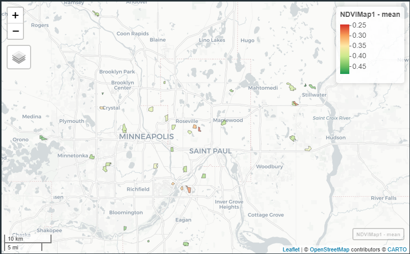
Figure 5: Final figure of mean NDVI isolated to only our study sites.
Data analysis
So, we have now collected some covariates, weather during the time of sampling and NDVI as a representation of greenness, as calculated using satellite imagery. These will be valuable for the analysis. The method used for the statsitical analysis will be extremely similar to that used in the Age Cohort analysis, also in this portfolio. In an effort to keep this write up as concise as possible, I will refer you there to learn about the techniques we (Kaylin Klecker and myself) used for model selection and auto correlation. Keep in mind in this analysis we will likely be dealing with spatial and temporal autocorrelation, as compared to only temporal autocorrelation in the other analysis.
You can view the full code at GitHub when it is publicly available.
References
Smitley, D., Hotchkiss, E., Buckley, K., Piombiono, M., Lewis, P., & Studyvin, J. (2022). Gradual Decline of Japanese Beetle (Coleoptera: Scarabaeidae) Populations in Michigan Follows Establishment of Ovavesicula popilliae (Microsporidia). Journal of Economic Entomology, 115(5), 1432-1441.
Cantwell, G. E. (1970). Standard methods for counting Nosema spores. Amer Bee J.
ANDREADIS, T. G., & HANULA, J. L. (1987). Ultrastructural Study and Description of Ovavesicula popilliae NG, N. Sp.(Microsporida: Pleistophoridae) from the Japanese Beetle, Popillia japonica (Coleoptera: Scarabaeidae) 1. The Journal of protozoology, 34(1), 15-21.